import matplotlib
if not hasattr(matplotlib.RcParams, "_get"):
    matplotlib.RcParams._get = dict.get

Backdoor Criterion

Setup

%%capture
%pip install dowhy==0.13 causaldata econml scikit-learn

import warnings
warnings.filterwarnings("ignore")

import pandas as pd
import numpy as np

from causaldata import nhefs
from sklearn.preprocessing import StandardScaler
from sklearn.linear_model import LogisticRegression, LinearRegression
from sklearn.ensemble import GradientBoostingRegressor

from dowhy import CausalModel
from econml.inference import BootstrapInference

• 금연이 체중 변화에 미치는 효과를 추정하고자 합니다.

• 이를 위해 NHEFS (National Health and Nutrition Examination Survey – Epidemiologic Follow-up Study) 데이터를 활용합니다.

• 이 데이터셋은 1971년 당시 흡연자였던 성인 코호트를 1982년까지 추적한 패널 자료로,
  금연 여부(qsmk, 1=금연, 0=계속 흡연), 체중 변화(wt82_71), 연령, 성별, 신체 활동 수준, 운동 습관 등 다양한 변수를 포함하고 있습니다.

df = nhefs.load_pandas().data.copy()

print("Shape of Data:")
print(df.shape)

print("Variable Names:")
print(df.columns)

df.head()

Shape of Data:
(1629, 67)
Variable Names:
Index(['seqn', 'qsmk', 'death', 'yrdth', 'modth', 'dadth', 'sbp', 'dbp', 'sex',
       'age', 'race', 'income', 'marital', 'school', 'education', 'ht', 'wt71',
       'wt82', 'wt82_71', 'birthplace', 'smokeintensity', 'smkintensity82_71',
       'smokeyrs', 'asthma', 'bronch', 'tb', 'hf', 'hbp', 'pepticulcer',
       'colitis', 'hepatitis', 'chroniccough', 'hayfever', 'diabetes', 'polio',
       'tumor', 'nervousbreak', 'alcoholpy', 'alcoholfreq', 'alcoholtype',
       'alcoholhowmuch', 'pica', 'headache', 'otherpain', 'weakheart',
       'allergies', 'nerves', 'lackpep', 'hbpmed', 'boweltrouble', 'wtloss',
       'infection', 'active', 'exercise', 'birthcontrol', 'pregnancies',
       'cholesterol', 'hightax82', 'price71', 'price82', 'tax71', 'tax82',
       'price71_82', 'tax71_82', 'id', 'censored', 'older'],
      dtype='object')

	seqn	qsmk	death	yrdth	modth	dadth	sbp	dbp	sex	age	...	hightax82	price71	price82	tax71	tax82	price71_82	tax71_82	id	censored	older
0	233.0	0.0	0.0	NaN	NaN	NaN	175.0	96.0	0	42.0	...	0.0	2.183594	1.739990	1.102295	0.461975	0.443787	0.640381	1	0.0	0.0
1	235.0	0.0	0.0	NaN	NaN	NaN	123.0	80.0	0	36.0	...	0.0	2.346680	1.797363	1.364990	0.571899	0.549316	0.792969	2	0.0	0.0
2	244.0	0.0	0.0	NaN	NaN	NaN	115.0	75.0	1	56.0	...	0.0	1.569580	1.513428	0.551270	0.230988	0.056198	0.320251	3	0.0	1.0
3	245.0	0.0	1.0	85.0	2.0	14.0	148.0	78.0	0	68.0	...	0.0	1.506592	1.451904	0.524902	0.219971	0.054794	0.304993	4	0.0	1.0
4	252.0	0.0	0.0	NaN	NaN	NaN	118.0	77.0	0	40.0	...	0.0	2.346680	1.797363	1.364990	0.571899	0.549316	0.792969	5	0.0	0.0

5 rows × 67 columns

• 처치변수: qsmk — 1982년 추적조사 시 금연 여부 (1=금연, 0=계속 흡연)

• 결과변수: wt82_71 — 체중 변화량(kg) = 1982년 체중 – 1971년 체중

• 통제변수:

  • sex: 성별 (0=남성, 1=여성)

  • age: baseline 만 나이

  • race: 인종 (0=백인, 1=기타)

  • education: 학력 수준 (5단계 범주)

  • smokeintensity: baseline 하루 평균 흡연량(개비)

  • smokeyrs: 흡연 지속 기간(년)

  • active: 일상생활 활동 수준 (3단계)

  • exercise: 여가시간 운동 수준 (3단계)

  • wt71: baseline 체중(kg)

treatment = "qsmk"
outcome = "wt82_71"

confounders = [
    "sex",
    "age",              
    "race",             
    "education",        
    "smokeintensity",   
    "smokeyrs",         
    "active",           
    "exercise",         
    "wt71"              
]

vars_needed = [treatment, outcome] + confounders
df_clean = df[vars_needed].dropna()

print("처치군/대조군:\n", df_clean[treatment].value_counts())

처치군/대조군:
 qsmk
0.0    1163
1.0     403
Name: count, dtype: int64

Model

gml_graph = """
graph [
  directed 1

  node [ id "qsmk" label "qsmk" ]
  node [ id "wt82_71" label "wt82_71" ]

  node [ id "sex" label "sex" ]
  node [ id "age" label "age" ]
  node [ id "race" label "race" ]
  node [ id "education" label "education" ]
  node [ id "smokeintensity" label "smokeintensity" ]
  node [ id "smokeyrs" label "smokeyrs" ]
  node [ id "active" label "active" ]
  node [ id "exercise" label "exercise" ]
  node [ id "wt71" label "wt71" ]

  edge [ source "sex" target "qsmk" ]
  edge [ source "sex" target "wt82_71" ]
  edge [ source "age" target "qsmk" ]
  edge [ source "age" target "wt82_71" ]
  edge [ source "race" target "qsmk" ]
  edge [ source "race" target "wt82_71" ]
  edge [ source "education" target "qsmk" ]
  edge [ source "education" target "wt82_71" ]
  edge [ source "smokeintensity" target "qsmk" ]
  edge [ source "smokeintensity" target "wt82_71" ]
  edge [ source "smokeyrs" target "qsmk" ]
  edge [ source "smokeyrs" target "wt82_71" ]
  edge [ source "active" target "qsmk" ]
  edge [ source "active" target "wt82_71" ]
  edge [ source "exercise" target "qsmk" ]
  edge [ source "exercise" target "wt82_71" ]
  edge [ source "wt71" target "qsmk" ]
  edge [ source "wt71" target "wt82_71" ]

  edge [ source "qsmk" target "wt82_71" ]
]
"""

cm = CausalModel(data=df_clean, treatment=treatment, outcome=outcome, graph=gml_graph)
cm.view_model(
    layout="dot"
)

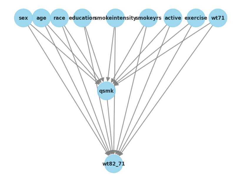
Identify

est_model = CausalModel(
    data=df_clean,
    treatment=treatment,
    outcome=outcome,
    graph=gml_graph
)

estimand = est_model.identify_effect()
print(estimand)

Estimand type: EstimandType.NONPARAMETRIC_ATE

### Estimand : 1
Estimand name: backdoor
Estimand expression:
   d                                                                           ↪
───────(E[wt_82_71|sex,age,smokeyrs,race,active,wt71,education,exercise,smokei ↪
d[qsmk]                                                                        ↪

↪           
↪ ntensity])
↪           
Estimand assumption 1, Unconfoundedness: If U→{qsmk} and U→wt82_71 then P(wt82_71|qsmk,sex,age,smokeyrs,race,active,wt71,education,exercise,smokeintensity,U) = P(wt82_71|qsmk,sex,age,smokeyrs,race,active,wt71,education,exercise,smokeintensity)

### Estimand : 2
Estimand name: iv
No such variable(s) found!

### Estimand : 3
Estimand name: frontdoor
No such variable(s) found!

### Estimand : 4
Estimand name: general_adjustment
Estimand expression:
   d                                                                           ↪
───────(E[wt_82_71|sex,age,smokeyrs,race,active,wt71,education,exercise,smokei ↪
d[qsmk]                                                                        ↪

↪           
↪ ntensity])
↪           
Estimand assumption 1, Unconfoundedness: If U→{qsmk} and U→wt82_71 then P(wt82_71|qsmk,sex,age,smokeyrs,race,active,wt71,education,exercise,smokeintensity,U) = P(wt82_71|qsmk,sex,age,smokeyrs,race,active,wt71,education,exercise,smokeintensity)

• Backdoor adjustment 가능
  모든 공변량을 조건화하면 qsmk → wt82_71 인과효과를 식별할 수 있습니다.

• IV, Front-door 전략 없음
  도구변수(Instrument)나 매개변수(Mediator)로 활용할 만한 변수가 존재하지 않습니다.

• 가정 (Unconfoundedness)
  관측되지 않은 잠재적 교란 변수(U)가 qsmk와 wt82_71 모두에 동시에 영향을 주지 않는다고 가정해야 합니다.

따라서 Back-door Adjustment를 통해 금연(qsmk)이 체중 변화(wt82_71)에 미치는 ATE를 추정할 수 있습니다.

Estimate

1. Linear Regression

estimate_lr = est_model.estimate_effect(
    identified_estimand=estimand,
    method_name="backdoor.linear_regression"
)
print("\n[ATE] Linear Regression:", estimate_lr.value)

[ATE] Linear Regression: 3.3811710339880823

2. Doubly Robust Learner

estimate_drl = est_model.estimate_effect(
    identified_estimand=estimand,
    method_name="backdoor.econml.dr.DRLearner",
    control_value=0,
    treatment_value=1,
    target_units="ate",
    confidence_intervals=True,
    method_params={
        "init_params": {
            "model_propensity": LogisticRegression(max_iter=5000),
            "model_regression": GradientBoostingRegressor(random_state=42)
        },
        "fit_params": {
            "inference": BootstrapInference(n_bootstrap_samples=500, n_jobs=-1)
        }
    }
)
print("[ATE] DR Learner:", estimate_drl.value)
print("[ATE] DR Learner 95% CI:", estimate_drl.get_confidence_intervals())

[ATE] DR Learner: 3.8479455513705227
[ATE] DR Learner 95% CI: [[[3.12167472]]

 [[5.29732315]]]

3. Double Machine Learning

estimate_dml = est_model.estimate_effect(
    identified_estimand=estimand,
    method_name="backdoor.econml.dml.DML",
    control_value=0,
    treatment_value=1,
    target_units="ate",
    confidence_intervals=True,
    method_params={
        "init_params": {
            "model_y": GradientBoostingRegressor(random_state=42),
            "model_t": GradientBoostingRegressor(random_state=42),
            "model_final": LinearRegression(fit_intercept=False),
        },
        "fit_params": {
            "inference": BootstrapInference(n_bootstrap_samples=500, n_jobs=-1)
        }
    }
)
print("[ATE] DML:", estimate_dml.value)
print("[ATE] DML 95% CI:", estimate_dml.get_confidence_intervals())

[ATE] DML: 3.8611289087159135
[ATE] DML 95% CI: [[[3.06774555]]

 [[5.17092571]]]

Refute

estimate_dml_fast = est_model.estimate_effect(
    identified_estimand=estimand,
    method_name='backdoor.econml.dml.DML',
    method_params={
        'init_params': {
            'model_y': GradientBoostingRegressor(random_state=42),
            'model_t': GradientBoostingRegressor(random_state=42),
            'model_final': LinearRegression(fit_intercept=False),
        },
        'fit_params': {}}
)
print("[ATE] DML:", estimate_dml.value)

[ATE] DML: 3.8611289087159135

1. Add Random Common Cause

데이터셋에 독립적인 무작위 변수를 넣었을 때, 추정값이 바뀌는가?

• 기대: New effect ≈ Estimated effect, p > 0.05

• 해석: 크게 변하면 → 모델이 잡음에 민감하거나 과적합일 가능성

res_random=est_model.refute_estimate(
    estimand,
    estimate_dml_fast,
    method_name="random_common_cause"
)
print(res_random)

Refute: Add a random common cause
Estimated effect:3.5111934415796173
New effect:3.4686090208687586
p value:0.72

2. Add Unobserved Common Cause

데이터에 관찰되지 않은 교란요인이 존재한다고 가정했을 때, 추정값이 얼마나 변하는가?

• 기대: New effect ≈ Estimated effect

• 해석:

  • 크게 변하지 않으면 → 잠재적 누락변수(confounder) 에도 견고(robust)

  • 크게 변하면 → 모델이 숨은 교란에 민감, 추가 변수 고려 필요

• 참고: 도메인 지식을 기반으로, 교란이 처리변수와 결과에 미치는 영향의 크기는 사용자가 직접 설정해야 합니다.

res_unobserved=est_model.refute_estimate(
    estimand,
    estimate_dml_fast,
    method_name="add_unobserved_common_cause",
    confounders_effect_on_treatment="linear",
    confounders_effect_on_outcome="linear",
    effect_strength_on_treatment=0.01,
    effect_strength_on_outcome=0.02
)
print(res_unobserved)

Refute: Add an Unobserved Common Cause
Estimated effect:3.5111934415796173
New effect:2.993841050044186

3. Placebo Treatment

처치 변수를 무작위로 섞인(permute) 가짜 처치(placebo)로 바꿨을 때, 추정값이 여전히 유의하게 나타나는가?

• 기대: New effect ≈ 0, p > 0.05

• 해석:

  • 효과가 사라지면 → 진짜 처치 효과만 반영된 것 → 견고(robust)

  • 여전히 유의하면 → 모델이 가짜 상관관계(spurious correlation) 를 잡고 있을 가능성

res_placebo=est_model.refute_estimate(
    estimand,
    estimate_dml_fast,
    method_name="placebo_treatment_refuter",
    placebo_type="permute",
    num_simulations=10
)
print(res_placebo)

Refute: Use a Placebo Treatment
Estimated effect:3.5111934415796173
New effect:0.14283539321647556
p value:0.3866345448655441

4. Use Subset of Data

데이터의 일부(예: 80%)만 무작위로 남겨두고 추정했을 때, 추정값이 얼마나 안정적인가?

• 기대: New effect ≈ Estimated effect, p > 0.05

• 해석:

  • 크게 변하지 않으면 → 표본 구성에 강건(robust)

  • 크게 변하면 → 특정 데이터 표본에 민감하거나, 과적합 가능성

res_subset=est_model.refute_estimate(
    estimand,
    estimate_dml_fast,
    method_name="data_subset_refuter",
    subset_fraction=0.8,
    num_simulations=10
)
print(res_subset)

Refute: Use a subset of data
Estimated effect:3.5111934415796173
New effect:3.4052136015402126
p value:0.4004970164482444